Just as we saw how to interact with the numpy and matplotlib libreries on python, this week we will explore another one so called SciPy for Scientific Python.
As this course is thought to be for scientist, these tools are particularly relevant.
SciPy is one library with some routines implemented specially for science.
It is divided
| Subpackage | Description |
|---|---|
| cluster | Clustering algorithms |
| constants | Physical and mathematical constants |
| fftpack | Fast Fourier Transforms routines |
| integrate | Integration and ODE solvers |
| interpolate | Interpolation and smoothing splines |
| Subpackage | Description |
|---|---|
| io | Input and Output |
| linag | Linear algebra |
| ndimage | N-dimensional image processing |
| ord | Orthogonal distance regression |
| optimize | Optimization and root-finding routines |
| Subpackage | Description |
|---|---|
| signal | Signal Processing |
| sparse | Sparse matrices and associated routines |
| spatial | Spatial data structures and algorithms |
| special | Special functions |
| stats | Statistical distributions and functions |
We can explore some of them in order to understand how libraries on python are used and how to read the docs!. SciPy Docs
During the course, everytime that we have used numpy, we have imported it with an alias, such as,
import numpy as np
And it allows us to use every part of numpy by using np. in front of the instruction, for instance np.pi or np.array()
scipy is constructed from different sub-modules, so it is not usually imported the same way numpy is. It is usual to import the submodules
from scipy import ASubModule
let us see a couple of examples, from the special submodule
One of the most widely used modules of scipy is the scipy.special because it allows us to use some special functions that are not easy to define by our own.
import numpy as np
import matplotlib.pylab as plt
from scipy import special
%config InlineBackend.figure_format = 'retina'
import matplotlib as mpl
mpl.rcParams['mathtext.fontset'] = 'cm'
Gamma function $\Gamma(z)$
Is a complex defined function, which correspond to the factorial for $z$ a real integer $$ \Gamma(z)=\int_{\infty}^{\infty} t^{z-1}e^{-t}dt $$
x=np.linspace(-5,5,1000)
y=special.gamma(x)
fig=plt.figure()
ax=fig.add_subplot(111)
ax.set_ylim(-5,7)
k = np.arange(1, 7)
for i in range(-5,1):
    ax.axvline(i,color='C1')
ax.plot(x,y,'.',label='Gamma function $\Gamma(x)$')

plt.plot(k, special.factorial(k-1),'^',color='C3',label='$n!$')
ax.grid()
plt.legend()

Airy Functions
Solution of
$$ \frac{d^2y(x)}{dx^2}-xy=0 $$x=np.linspace(-15,2.5,1000)
ai, aip, bi, bip=special.airy(x)
fig=plt.figure(figsize=(10,5))
ax1=fig.add_subplot(221)
ax1.plot(x,ai,label='$A_i(x)$')
ax1.plot(x,aip,label="$A'_i(x)$")
ax1.grid()
plt.legend()
ax2=fig.add_subplot(222)
ax2.plot(x,bi,label="$B_i(x)$")
ax2.plot(x,bip,label="$B'_i(x)$")
ax2.grid()
plt.legend()
ax3=fig.add_subplot(212)
ax3.set_ylim(-.5,1)
ax3.plot(x,ai,label="$A_i(x)$")
ax3.plot(x,bi,label="$B_i(x)$")
ax3.grid()
plt.legend()

$\text{erf}(x)$ Function
Very important in probability, due to it is the truncated integral of a gaussian.
$$ \text{erf}(x)=\frac{2}{\sqrt{\pi}}\int^x_0e^{-t^2}dt $$x=np.linspace(-5,5,1000)
y=special.erf(x)
fig=plt.figure()
ax=fig.add_subplot(111)
ax.plot(x,y,label='erf$(x)$')
ax.grid()
plt.legend()
plt.show()

Special Polynomials
There are some polynimial families which were found while looking for solution for some EDO. Here we are going to see some of them WITHOUT talking about their properties.
Legendre Polynomials
Solution of the Legendre equation $$ \frac{d}{dx}\left[(1-x^2)\frac{dP_n(x)}{dx}\right]+n(n+1)P_n(x)=0 $$
This equation becomes of interest when solving the Laplace equation on spherical coordinates.
$$\nabla^2\varphi(\mathbf{r})=0$$That means, all the electrostatic and magetostatic.
x=np.linspace(-1,1,1000)
for i in range(10):
    y=special.legendre(i)
    plt.plot(x,y(x))
plt.show()

Laguerre Polynomials
Solution of the Laguerre equation $$ x\frac{d^2L_n(x)}{dx^2}+(1-x)\frac{dL_n(x)}{dx}+nL_n(x)=0 $$
They arise in quantum mechanics on several problems,
- The radial equation of the Schrödinger equation for a single electron atom (Hydrogen).
- The static Wigner functions of oscillator systems in quantum mechanics in phase space.
- Solution for the Morse potential and of the 3D isotropic harmonic oscillator.
x=np.linspace(-5,20,1000)
fig=plt.figure(figsize=(10,5))
ax1=fig.add_subplot(121)
ax2=fig.add_subplot(122)
for i in range(5):
    y=special.laguerre(i)
    ax1.plot(x,y(x),label=str(i))
    ax1.set_ylim(-20,20)
    ax2.plot(x,y(x),label=str(i))
ax1.legend()
ax2.legend()
plt.show()

Hermite Polynomials
Solution of the Hermite equation $$ H_n(x)=(-1)^ne^{x^2}\frac{d^n}{dx^n}e^{-x^2} $$
Solution of the quantum harmonic oscillator.
x=np.linspace(-3,3,1000)
fig=plt.figure(figsize=(10,5))
ax1=fig.add_subplot(121)
ax2=fig.add_subplot(122)
for i in range(5):
    y=special.hermite(i)
    ax1.plot(x,y(x),label=str(i))
    ax1.set_ylim(-40,80)
    ax2.plot(x,y(x),label=str(i))
ax1.legend()
ax2.legend()
plt.show()

Chebyshev Polynomials (First Kind)
Are defined to be solution of $$ (1-x^2)\frac{d^2}{dx^2}T_n(x)-x\frac{d}{dx}T_n(x)+n^2+T_n(x)=0 $$
x=np.linspace(-1,1,1000)
for i in range(5):
    y=special.chebyt(i)
    plt.plot(x,y(x))
plt.show()

Regression Analysis!!
One of the most important applications of programming on science is the data analysis.
This analysis may vary depending the area, but if we restrict ourselves to the experiments, the measurements used to test models and theories.
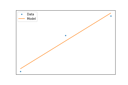
How can we know if our data follows a particular model?.For example, we he have collected a set of data, and we want to know if it follows a straight line (That is our model), the question here splits into two parts
- Finding a unique line that describes the data given some criteria.
- Evaluating how good this line describes the data.
What can be a good criteria?
As we want to find a unique curve that describes the data, we must have some criteria so that the result choosen is the best according the criteria.
Least Squares Criteria
Least Squares Criteria
Least Squares Criteria
Least Squares Criteria

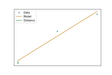
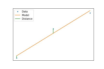
So the best line is the one that minimizes the vertical distance
$$ \min_{\mathbf{\alpha}}\left(\sum_i(f(x_i,\mathbf{\alpha})-y_i)^2\right) $$When we have a linear model, this minimization can be calculated using a formula, such that $$ f(x)=ax+b $$
where the parameters can be calculated as,
$$ a=\frac{\sum_i y_i\sum_i(x^2_i)-\sum_ix_i\sum_i(x_iy_i)}{N\sum_i(x^2_i)-(\sum_i x_i)^2} $$and $$ b=\frac{N\sum_i (x_iy_i)-\sum_ix_i\sum_iy_i}{N\sum_i(x^2_i)-(\sum_i x_i)^2} $$
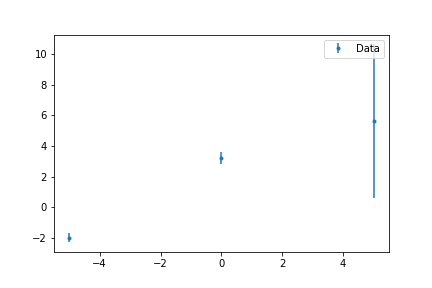
Experimental data
Have error bars!, that means that
- Data with small error weights more
- Data with big error weights less
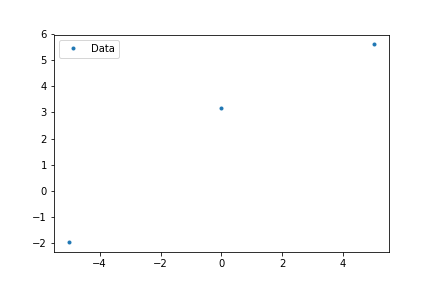
How can we use these ideas with python?.
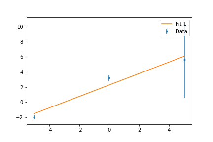
There are several ways, but we are going to concentrate on one very robust method of SciPy, curve_fit.
x,y,err=np.genfromtxt('https://raw.githubusercontent.com/jmsevillam/Herramientas-Computacionales-UniAndes/master/Data/data_fit.dat')
fig=plt.figure()
ax=fig.add_subplot(111)
ax.plot(x,y,'.',label='data')
plt.legend()
plt.show()

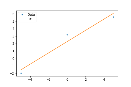
from scipy.optimize import curve_fit
def fit(x,a,b):
    return a*x+b
popt,pcov=curve_fit(fit,x,y)
fig=plt.figure()
ax=fig.add_subplot(111)
ax.plot(x,y,'.',label='data')
ax.plot(x,fit(x,*popt),'-',label='data')
plt.legend()
plt.show()

print(popt,pcov.diagonal()**0.5)
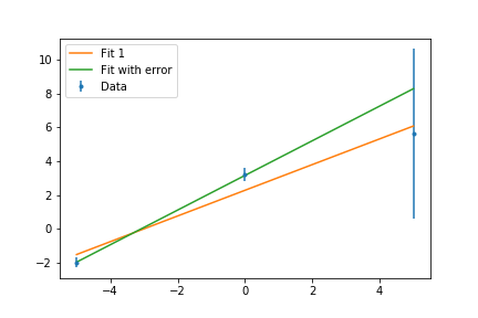
popt2,pcov2=curve_fit(fit,x,y,sigma=err)
print(popt2,pcov2.diagonal()**0.5)
fig=plt.figure()
ax=fig.add_subplot(111)
ax.errorbar(x,y,err,fmt='.',label='Data')
ax.plot(x,fit(x,*popt),'-',label='Fit')
ax.plot(x,fit(x,*popt2),'-',label='Fit with Errorbars')
plt.legend()
plt.show()

print(popt,pcov.diagonal()**0.5,popt2,pcov2.diagonal()**0.5)