We are almost finished with our course!
So now, we are ready to apply all the tools we have developed so far.
This week, we will see how can use code to solve mathematical problems such as,
- Derivate functions.
- Integrate functions (Definited integrals).
- Root searching.
We will use the libraries available on python we have worked on last weeks (NumPy and Matplotlib).
Theory
Searching roots of a function is one of the most common problems solved with computers on science. So we are going to learn two of the most widely used methods,
- Bisection
- Newton-Raphson
The method work as follows.
- We select the two points of the interval (the limits).
- Calculate the middle point.
- Calculate the function on the midpont.
- Define the convergence
- The interval is small enough.
- The value of the function on the midpoint is small enough.
- If the criteria are not satisfied, check the signs,
- If $f(a_n)>0$ and $f(p_n)>0$ or $f(a_n)<0$ and $f(p_n)<0$, then the root is now on $(p_n,b_n]$.
- If $f(a_n)<0$ and $f(p_n)>0$ or If $f(a_n)>0$ and $f(p_n)<0$, then the root is now on $(a_n,p_n]$.
- Repeat for the new limits.
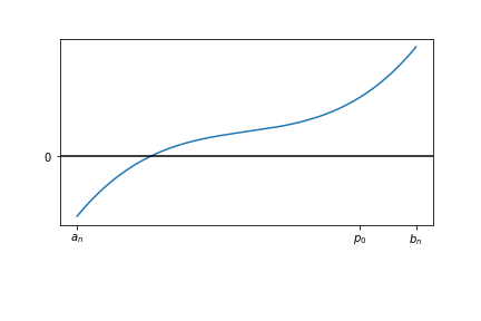
Function
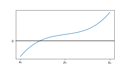
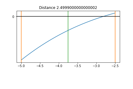
Initial Interval
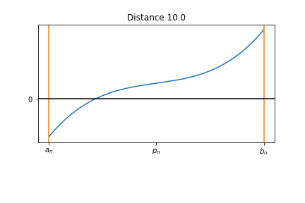
Midpoint
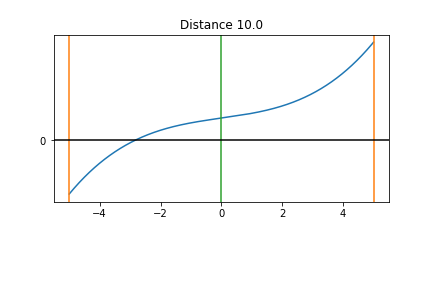
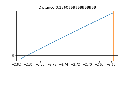
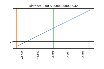
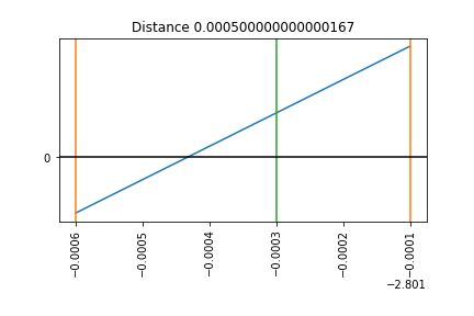
Resize the Interval step 1
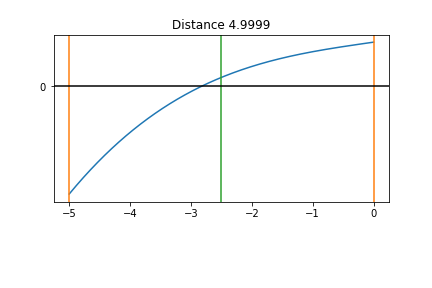
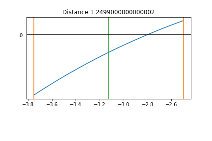
Resize the Interval step 2
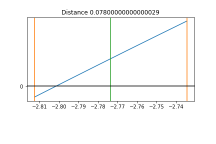
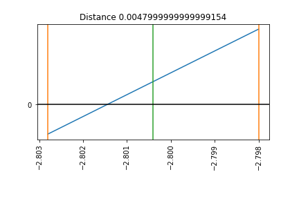
Resize the Interval step 3
Resize the Interval step 4
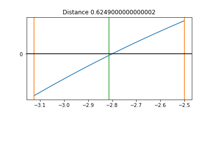
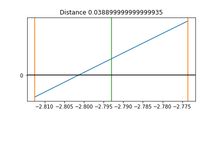
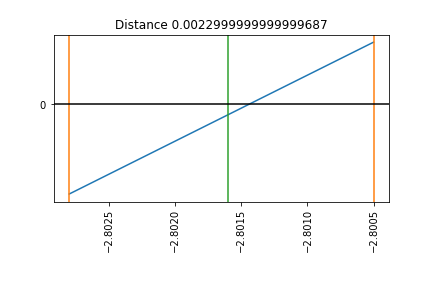
Resize the Interval step 5
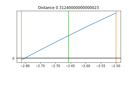
Resize the Interval step 6
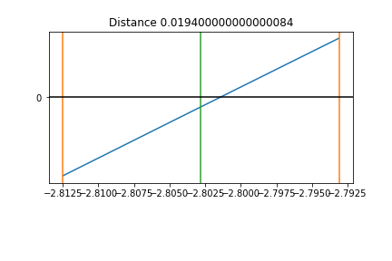
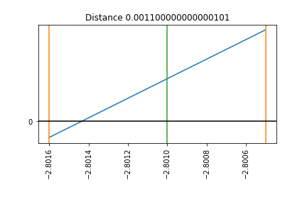
Resize the Interval step 7
Resize the Interval step 8
Resize the Interval step 9
Resize the Interval
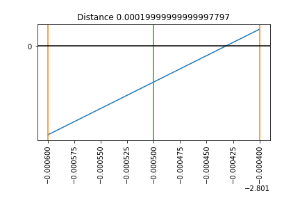
Resize the Interval step 10
Resize the Interval step 11
Resize the Interval step 12
Resize the Interval step 13
Resize the Interval step 14
The first problem we will solve, is finding the value of $x$ such that $f(x)=0$ with
$$ f(x)=\left(\tanh\left(\frac{x}{4}\right)+\frac{\cos(x)\sin(x)}{x}\right)^3 $$import numpy as np
import matplotlib.pylab as plt
def f(x):
    return (np.tanh(0.25*x)+(np.cos(x)*np.sin(x))/x)**3
x=np.linspace(-10,10,100)
y=f(x)
fig=plt.figure()
ax=fig.add_subplot(111)
ax.plot(x,y)
ax.axhline(0,color='C1')

def bisec(f,an,bn):
    eps=1e-10
    while (np.abs(an-bn)>eps):
        pm=(an+bn)/2.
        if (f(an)*f(pm)>0):
            an=pm
        else:
            bn=pm
    return pm
print(bisec(f,-10,10.1),f(bisec(f,-10,10.1)))
The first problem we will solve, is finding the value of $x$ such that $f(x)=0$ with
$$ f(x)=\tanh\left(x-2.1\right)+0.1 $$def f(x0):
return np.tanh(x0-2.1)+0.1
x=np.linspace(-10,10,100)
y=f(x)
fig=plt.figure()
ax=fig.add_subplot(111)
ax.plot(x,y)
ax.axhline(0,color='C1')

print(bisec(f,-10,10.1),f(bisec(f,-10,10.1)))
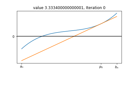
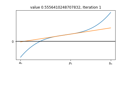
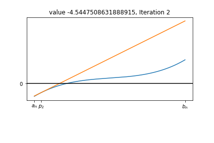
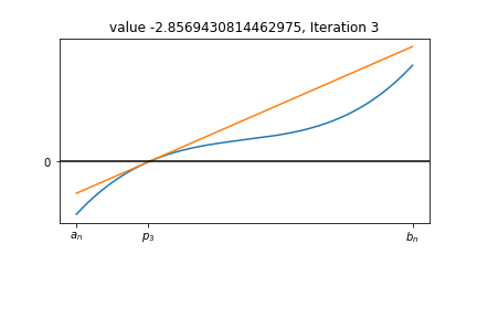
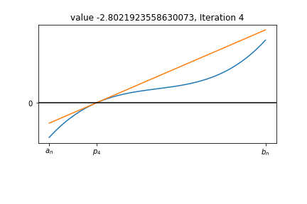
Newton
This method is more complex but precise than the bisection. This is also known as the tangent method, because it starts from a guess and moves as the tangent line.
The method work as follows.
We select an initial guess $p_0$, then the following point is found by taking the zero of the derivative on that point. The equation of that line is $$y=f'(p_0)(x_1-x_0)+f(x_0).$$
So, in order to find the value of $x_1$, $y=0$, that leads to $$ x_{i+1}=x_{i}-\frac{f(x_i)}{f'(x_i)}, $$ and it is repeated until a tolerance. (Or $f(x_i)==0$).
Function
Initial Interval
Midpoint
Resize the Interval step 1
Resize the Interval step 2
Resize the Interval step 3
Resize the Interval step 4
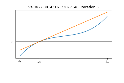
Resize the Interval step 5

Resize the Interval step 6

Resize the Interval step 7

def Newton(f0,df0,xi):
    eps=1e-10
    while np.abs(f0(xi))>eps:
        xi-=f0(xi)/df0(xi)
    return xi
Again the first function we are testing
$$ f(x)=\left(\tanh\left(\frac{x}{4}\right)+\frac{\cos(x)\sin(x)}{x}\right)^3 $$def f(x):
return (np.tanh(0.25*x)+(np.cos(x)*np.sin(x))/x)**3
x=np.linspace(-10,10,100)
y=f(x)
fig=plt.figure()
ax=fig.add_subplot(111)
ax.plot(x,y)
ax.axhline(0,color='C1')
def df(x):
    return (0.75/x**4)*((x*np.tanh(0.25*x)+
                         np.sin(x)*np.cos(x))**2.)*(x*x*(np.cosh(0.25*x))**-2.
                                                                      -4*x*np.sin(x)**2+4*x*np.cos(x)**2.-4*np.cos(x)*np.sin(x))
print(bisec(f,-10,10.1),Newton(f,df,0.5))
def f1(x0):
    return np.tanh(x0-2.1)+0.1
def df1(x0):
    return 1./np.cosh(x0-2.1)**2.
x=np.linspace(-10,10,100)
y=f1(x)
fig=plt.figure()
ax=fig.add_subplot(111)
ax.plot(x,y)
ax.axhline(0,color='C1')
print(bisec(f1,-10,10.1),Newton(f1,df1,1.5))
But, what if we consider a different initial condition?
print(bisec(f1,-10,10.1),Newton(f1,df1,10.0))