imagen


Pandas


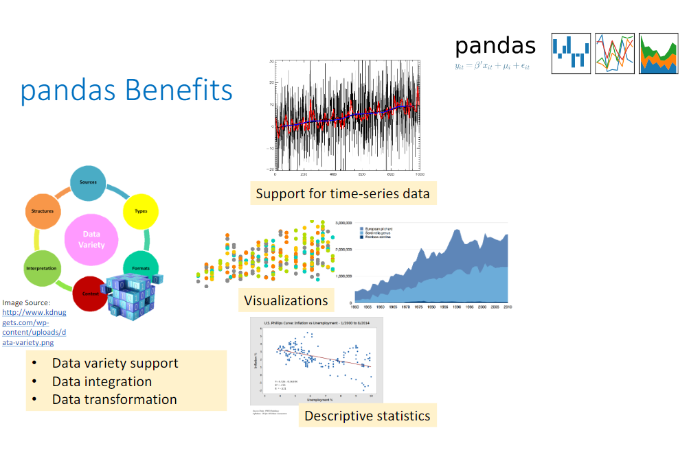
pandas is a Python library for data analysis. It offers a number of data exploration, cleaning and transformation operations that are critical in working with data in Python.

pandas build upon numpy and scipy providing easy-to-use data structures and data manipulation functions with integrated indexing.

The main data structures pandas provides are Series and DataFrames. After a brief introduction to these two data structures and data ingestion, the key features of pandas this notebook covers are:

  • Generating descriptive statistics on data
  • Data cleaning using built in pandas functions
  • Frequent data operations for subsetting, filtering, insertion, deletion and aggregation of data
  • Merging multiple datasets using dataframes
  • Working with timestamps and time-series data

Additional Recommended Resources:

Let's get started with our first pandas notebook!

In [1]:
import pandas as pd

Introduction to pandas Data Structures


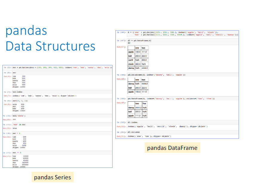
*pandas* has two main data structures it uses, namely, *Series* and *DataFrames*.

pandas Series

pandas Series one-dimensional labeled array.

imagen_2

In [2]:
ser = pd.Series([100, 'foo', 300, 'bar', 500], ['tom', 'bob', 'nancy', 'dan', 'eric'])
print(ser)
tom      100
bob      foo
nancy    300
dan      bar
eric     500
dtype: object
In [3]:
ser.index
Out[3]:
Index(['tom', 'bob', 'nancy', 'dan', 'eric'], dtype='object')
In [4]:
ser.loc[['nancy','bob']]
Out[4]:
nancy    300
bob      foo
dtype: object
In [5]:
ser[[4, 3, 1]]
Out[5]:
eric    500
dan     bar
bob     foo
dtype: object
In [6]:
ser.iloc[2]
Out[6]:
300
In [7]:
'bob' in ser
Out[7]:
True
In [8]:
print(ser)
print(ser*2)
tom      100
bob      foo
nancy    300
dan      bar
eric     500
dtype: object
tom         200
bob      foofoo
nancy       600
dan      barbar
eric       1000
dtype: object
In [9]:
ser[['nancy', 'eric']] ** 2
Out[9]:
nancy     90000
eric     250000
dtype: object

pandas DataFrame

pandas DataFrame is a 2-dimensional labeled data structure.

Create DataFrame from dictionary of Python Series

In [10]:
d = {'one' : pd.Series([100., 200., 300.], index=['apple', 'ball', 'clock']),
     'two' : pd.Series([111., 222., 333., 4444.], index=['apple', 'ball', 'cerill', 'dancy'])}
df = pd.DataFrame(d)
In [11]:
df
Out[11]:
one two
apple 100.0 111.0
ball 200.0 222.0
cerill NaN 333.0
clock 300.0 NaN
dancy NaN 4444.0

Other way to do the same

In [12]:
d = {'one' : [100., 200.,float("NaN"), 300., float("NaN")],'two':[111., 222., 333., float("NaN"),4444.],"tmp_index":['apple', 'ball', 'cerill', 'clock', 'dancy']}
df=pd.DataFrame(data=d)
df.set_index("tmp_index",inplace=True)
df.index.name = None
df
Out[12]:
one two
apple 100.0 111.0
ball 200.0 222.0
cerill NaN 333.0
clock 300.0 NaN
dancy NaN 4444.0
In [13]:
d = {'one' : pd.Series([100., 200., 300.], index=['apple', 'ball', 'clock']),
     'two' : pd.Series([111., 222., 333., 4444.], index=['apple', 'ball', 'cerill', 'dancy'])}
df = pd.DataFrame(d)
pd.DataFrame(d, index=['dancy', 'ball', 'apple'])
Out[13]:
one two
dancy NaN 4444.0
ball 200.0 222.0
apple 100.0 111.0
In [14]:
pd.DataFrame(d, index=['dancy', 'ball', 'apple'], columns=['two', 'five'])
Out[14]:
two five
dancy 4444.0 NaN
ball 222.0 NaN
apple 111.0 NaN

Create DataFrame from list of Python dictionaries

In [15]:
data = [{'alex': 1, 'joe': 2}, {'ema': 5, 'dora': 10, 'alice': 20}]
In [16]:
pd.DataFrame(data)
Out[16]:
alex alice dora ema joe
0 1.0 NaN NaN NaN 2.0
1 NaN 20.0 10.0 5.0 NaN
In [17]:
pd.DataFrame(data, index=['orange', 'red'])
Out[17]:
alex alice dora ema joe
orange 1.0 NaN NaN NaN 2.0
red NaN 20.0 10.0 5.0 NaN
In [18]:
pd.DataFrame(data, columns=['joe', 'dora','alice'])
Out[18]:
joe dora alice
0 2.0 NaN NaN
1 NaN 10.0 20.0

Basic DataFrame operations

In [19]:
df
Out[19]:
one two
apple 100.0 111.0
ball 200.0 222.0
cerill NaN 333.0
clock 300.0 NaN
dancy NaN 4444.0
In [20]:
df['one']
Out[20]:
apple     100.0
ball      200.0
cerill      NaN
clock     300.0
dancy       NaN
Name: one, dtype: float64
In [21]:
df['three'] = df['one'] * df['two']
df
Out[21]:
one two three
apple 100.0 111.0 11100.0
ball 200.0 222.0 44400.0
cerill NaN 333.0 NaN
clock 300.0 NaN NaN
dancy NaN 4444.0 NaN
In [22]:
df['flag'] = df['one'] > 250
df
Out[22]:
one two three flag
apple 100.0 111.0 11100.0 False
ball 200.0 222.0 44400.0 False
cerill NaN 333.0 NaN False
clock 300.0 NaN NaN True
dancy NaN 4444.0 NaN False
In [23]:
three = df.pop('three')
three
Out[23]:
apple     11100.0
ball      44400.0
cerill        NaN
clock         NaN
dancy         NaN
Name: three, dtype: float64
In [24]:
df
Out[24]:
one two flag
apple 100.0 111.0 False
ball 200.0 222.0 False
cerill NaN 333.0 False
clock 300.0 NaN True
dancy NaN 4444.0 False
In [25]:
del df['two']
In [26]:
df
Out[26]:
one flag
apple 100.0 False
ball 200.0 False
cerill NaN False
clock 300.0 True
dancy NaN False
In [27]:
df.insert(2, 'copy_of_one', df['one'])
df
Out[27]:
one flag copy_of_one
apple 100.0 False 100.0
ball 200.0 False 200.0
cerill NaN False NaN
clock 300.0 True 300.0
dancy NaN False NaN
In [28]:
df['one_upper_half'] = df['one'][:2]
df
Out[28]:
one flag copy_of_one one_upper_half
apple 100.0 False 100.0 100.0
ball 200.0 False 200.0 200.0
cerill NaN False NaN NaN
clock 300.0 True 300.0 NaN
dancy NaN False NaN NaN
In [29]:
df.dropna(axis=0,thresh=2)
Out[29]:
one flag copy_of_one one_upper_half
apple 100.0 False 100.0 100.0
ball 200.0 False 200.0 200.0
clock 300.0 True 300.0 NaN

Case Study: Movie Data Analysis


This notebook uses a dataset from the MovieLens website. We will describe the dataset further as we explore with it using pandas.

Download the Dataset

Please note that you will need to download the dataset.

Here are the links to the data source and location:

Once the download completes, please make sure the data files are in a directory called movielens

Let us look at the files in this dataset using the UNIX command ls.

In [30]:
%%bash
ls movielens/Large/
README.txt
genome-scores.csv
genome-tags.csv
links.csv
movies.csv
ratings.csv
tags.csv
In [31]:
%%bash
cat movielens/Large/movies.csv | wc -l
27279
In [32]:
%%bash
cat movielens/Large/ratings.csv | wc -l
20000264
In [33]:
%%bash
head -5 ./movielens/Large/ratings.csv
userId,movieId,rating,timestamp
1,2,3.5,1112486027
1,29,3.5,1112484676
1,32,3.5,1112484819
1,47,3.5,1112484727

Use Pandas to Read the Dataset


In this notebook, we will be using three CSV files:

  • ratings.csv : userId,movieId,rating, timestamp
  • tags.csv : userId,movieId, tag, timestamp
  • movies.csv : movieId, title, genres

Using the read_csv function in pandas, we will ingest these three files.

In [34]:
movies = pd.read_csv('./movielens/Large/movies.csv', sep=',')
print(type(movies))
movies.head(15)
<class 'pandas.core.frame.DataFrame'>
Out[34]:
movieId title genres
0 1 Toy Story (1995) Adventure|Animation|Children|Comedy|Fantasy
1 2 Jumanji (1995) Adventure|Children|Fantasy
2 3 Grumpier Old Men (1995) Comedy|Romance
3 4 Waiting to Exhale (1995) Comedy|Drama|Romance
4 5 Father of the Bride Part II (1995) Comedy
5 6 Heat (1995) Action|Crime|Thriller
6 7 Sabrina (1995) Comedy|Romance
7 8 Tom and Huck (1995) Adventure|Children
8 9 Sudden Death (1995) Action
9 10 GoldenEye (1995) Action|Adventure|Thriller
10 11 American President, The (1995) Comedy|Drama|Romance
11 12 Dracula: Dead and Loving It (1995) Comedy|Horror
12 13 Balto (1995) Adventure|Animation|Children
13 14 Nixon (1995) Drama
14 15 Cutthroat Island (1995) Action|Adventure|Romance
In [35]:
tags = pd.read_csv('./movielens/Large/tags.csv', sep=',')
tags.head()
Out[35]:
userId movieId tag timestamp
0 18 4141 Mark Waters 1240597180
1 65 208 dark hero 1368150078
2 65 353 dark hero 1368150079
3 65 521 noir thriller 1368149983
4 65 592 dark hero 1368150078
In [36]:
ratings = pd.read_csv('./movielens/Large/ratings.csv', sep=',', parse_dates=['timestamp'])
ratings.head()
Out[36]:
userId movieId rating timestamp
0 1 2 3.5 1112486027
1 1 29 3.5 1112484676
2 1 32 3.5 1112484819
3 1 47 3.5 1112484727
4 1 50 3.5 1112484580

For current analysis, we will remove the Timestamp ( we could get to it later if you want)


In [37]:
del ratings['timestamp']
del tags['timestamp']

Data Structures

Series

In [38]:
row_0 = tags.iloc[0]
print(type(row_0))
print(row_0)
<class 'pandas.core.series.Series'>
userId              18
movieId           4141
tag        Mark Waters
Name: 0, dtype: object
In [39]:
row_0.index
Out[39]:
Index(['userId', 'movieId', 'tag'], dtype='object')
In [40]:
row_0['userId']
Out[40]:
18
In [41]:
'rating' in row_0
Out[41]:
False
In [42]:
row_0.name
Out[42]:
0
In [43]:
row_0 = row_0.rename('first_row')
row_0.name
Out[43]:
'first_row'

Descriptive Statistics

Let's look how the ratings are distributed!

In [44]:
ratings.describe()
Out[44]:
userId movieId rating
count 2.000026e+07 2.000026e+07 2.000026e+07
mean 6.904587e+04 9.041567e+03 3.525529e+00
std 4.003863e+04 1.978948e+04 1.051989e+00
min 1.000000e+00 1.000000e+00 5.000000e-01
25% 3.439500e+04 9.020000e+02 3.000000e+00
50% 6.914100e+04 2.167000e+03 3.500000e+00
75% 1.036370e+05 4.770000e+03 4.000000e+00
max 1.384930e+05 1.312620e+05 5.000000e+00
In [45]:
ratings.mode()
Out[45]:
userId movieId rating
0 118205 296 4.0
In [46]:
ratings.corr()
Out[46]:
userId movieId rating
userId 1.000000 -0.000850 0.001175
movieId -0.000850 1.000000 0.002606
rating 0.001175 0.002606 1.000000
In [47]:
filter_2 = ratings.loc[ratings['rating'] > 0]
In [48]:
filter_2.groupby("movieId").mean()
Out[48]:
userId rating
movieId
1 69282.396821 3.921240
2 69169.928202 3.211977
3 69072.079388 3.151040
4 69652.913280 2.861393
5 69113.475454 3.064592
6 69226.328633 3.834930
7 69100.961809 3.366484
8 68677.092580 3.142049
9 70310.064899 3.004924
10 69161.741045 3.430029
11 69529.290717 3.667713
12 69245.668661 2.619766
13 70136.308693 3.272416
14 69468.605945 3.432082
15 69273.411684 2.721993
16 68817.899103 3.787455
17 69093.916727 3.968573
18 69830.091293 3.373631
19 69367.608129 2.607412
20 69822.326151 2.880754
21 69448.155374 3.581689
22 68741.821011 3.319400
23 70304.317176 3.148235
24 68901.418517 3.199849
25 69241.775855 3.689510
26 70215.360799 3.628857
27 67274.806943 3.413520
28 69610.200698 4.057546
29 69010.756925 3.952230
30 70776.333333 3.633880
... ... ...
131146 79570.000000 4.000000
131148 79570.000000 4.000000
131150 79570.000000 4.000000
131152 74937.000000 0.500000
131154 79570.000000 3.500000
131156 79570.000000 4.000000
131158 108819.000000 4.000000
131160 79570.000000 4.000000
131162 42229.000000 2.000000
131164 54560.000000 4.000000
131166 54560.000000 4.000000
131168 64060.000000 3.500000
131170 95841.000000 3.500000
131172 128309.000000 1.000000
131174 109286.000000 3.500000
131176 109286.000000 4.500000
131180 117144.000000 2.500000
131231 63046.000000 3.500000
131237 134701.000000 3.000000
131239 79570.000000 4.000000
131241 79570.000000 4.000000
131243 79570.000000 4.000000
131248 79570.000000 4.000000
131250 79570.000000 4.000000
131252 79570.000000 4.000000
131254 79570.000000 4.000000
131256 79570.000000 4.000000
131258 28906.000000 2.500000
131260 65409.000000 3.000000
131262 133047.000000 4.000000

26744 rows × 2 columns

Data Cleaning: Handling Missing Data

In [49]:
movies.shape
Out[49]:
(27278, 3)

Is there any row Null?

In [50]:
movies.isnull().any()
Out[50]:
movieId    False
title      False
genres     False
dtype: bool

Nice!!, so we do not have to worry about this!

In [51]:
ratings.shape
Out[51]:
(20000263, 3)
In [52]:
ratings.isnull().any()
Out[52]:
userId     False
movieId    False
rating     False
dtype: bool

Nice!!, so we do not have to worry about this!

In [53]:
tags.shape
Out[53]:
(465564, 3)
In [54]:
tags.isnull().any()
Out[54]:
userId     False
movieId    False
tag         True
dtype: bool

Unfortunately we will have to deal with NaN values in this data set

In [55]:
tags = tags.dropna()

We check agaiin if there is any row null

In [56]:
tags.isnull().any()
Out[56]:
userId     False
movieId    False
tag        False
dtype: bool

Thats nice! Nonetheless, notice that the number of lines have reduced.

In [57]:
tags.shape
Out[57]:
(465548, 3)

Data Visualization

In [58]:
import matplotlib.pylab as plt
In [59]:
ratings.hist(column='rating', figsize=(15,10),bins=10)
plt.show()

Getting information from columns

In [60]:
tags['tag'].head()
Out[60]:
0      Mark Waters
1        dark hero
2        dark hero
3    noir thriller
4        dark hero
Name: tag, dtype: object
In [61]:
movies[['title','genres']].head()
Out[61]:
title genres
0 Toy Story (1995) Adventure|Animation|Children|Comedy|Fantasy
1 Jumanji (1995) Adventure|Children|Fantasy
2 Grumpier Old Men (1995) Comedy|Romance
3 Waiting to Exhale (1995) Comedy|Drama|Romance
4 Father of the Bride Part II (1995) Comedy
In [62]:
ratings[-10:]
Out[62]:
userId movieId rating
20000253 138493 60816 4.5
20000254 138493 61160 4.0
20000255 138493 65682 4.5
20000256 138493 66762 4.5
20000257 138493 68319 4.5
20000258 138493 68954 4.5
20000259 138493 69526 4.5
20000260 138493 69644 3.0
20000261 138493 70286 5.0
20000262 138493 71619 2.5
In [63]:
ratings.tail(10)
Out[63]:
userId movieId rating
20000253 138493 60816 4.5
20000254 138493 61160 4.0
20000255 138493 65682 4.5
20000256 138493 66762 4.5
20000257 138493 68319 4.5
20000258 138493 68954 4.5
20000259 138493 69526 4.5
20000260 138493 69644 3.0
20000261 138493 70286 5.0
20000262 138493 71619 2.5
In [64]:
tag_counts = tags['tag'].value_counts()
tag_counts.head().plot(kind='bar', figsize=(12,8))
Out[64]:
<matplotlib.axes._subplots.AxesSubplot at 0x26381863b38>
In [65]:
tag_counts.head(60).plot(kind='bar', figsize=(12,8))
Out[65]:
<matplotlib.axes._subplots.AxesSubplot at 0x26380380710>
In [66]:
tag_counts[60:100].plot(kind='bar', figsize=(12,8))
Out[66]:
<matplotlib.axes._subplots.AxesSubplot at 0x26381902780>

Filters for Selecting Rows

In [67]:
is_highly_rated = ratings['rating'] >= 4.0
ratings[is_highly_rated].head()
Out[67]:
userId movieId rating
6 1 151 4.0
7 1 223 4.0
8 1 253 4.0
9 1 260 4.0
10 1 293 4.0
In [68]:
is_animation = movies['genres'].str.contains('Animation')
movies[is_animation].head(15)
Out[68]:
movieId title genres
0 1 Toy Story (1995) Adventure|Animation|Children|Comedy|Fantasy
12 13 Balto (1995) Adventure|Animation|Children
47 48 Pocahontas (1995) Animation|Children|Drama|Musical|Romance
236 239 Goofy Movie, A (1995) Animation|Children|Comedy|Romance
241 244 Gumby: The Movie (1995) Animation|Children
310 313 Swan Princess, The (1994) Animation|Children
360 364 Lion King, The (1994) Adventure|Animation|Children|Drama|Musical|IMAX
388 392 Secret Adventures of Tom Thumb, The (1993) Adventure|Animation
547 551 Nightmare Before Christmas, The (1993) Animation|Children|Fantasy|Musical
553 558 Pagemaster, The (1994) Action|Adventure|Animation|Children|Fantasy
582 588 Aladdin (1992) Adventure|Animation|Children|Comedy|Musical
588 594 Snow White and the Seven Dwarfs (1937) Animation|Children|Drama|Fantasy|Musical
589 595 Beauty and the Beast (1991) Animation|Children|Fantasy|Musical|Romance|IMAX
590 596 Pinocchio (1940) Animation|Children|Fantasy|Musical
604 610 Heavy Metal (1981) Action|Adventure|Animation|Horror|Sci-Fi
In [69]:
ratings_count = ratings[['movieId','rating']].groupby('rating').count()
ratings_count
Out[69]:
movieId
rating
0.5 239125
1.0 680732
1.5 279252
2.0 1430997
2.5 883398
3.0 4291193
3.5 2200156
4.0 5561926
4.5 1534824
5.0 2898660

Group By and Aggregate

In [70]:
average_rating = ratings[['movieId','rating']].groupby('movieId').mean() # We are not interested in the user that voted for it
average_rating.head()
Out[70]:
rating
movieId
1 3.921240
2 3.211977
3 3.151040
4 2.861393
5 3.064592

Task:

Get the movies that are in average the best rated movies

Option 1:

Sort the list in descending order and get the first rows

In [71]:
sorted_average_rating=average_rating.sort_values(by="rating",ascending=False)
sorted_average_rating.head()
Out[71]:
rating
movieId
95517 5.0
105846 5.0
89133 5.0
105187 5.0
105191 5.0

Option 2:

Do not sort the list but intead ask where we have that the rating score is $5.0$

In [72]:
average_rating.loc[average_rating.rating==5.0].head()
Out[72]:
rating
movieId
26718 5.0
27914 5.0
32230 5.0
40404 5.0
54326 5.0

But since we do not understand to what this Id movie is related, we would like to see intead the name of the movie. To do that, we need to see in the movies DataFrame

In [73]:
id_movie=average_rating.loc[average_rating.rating==5.0].index
In [74]:
movies.loc[movies.movieId.isin(id_movie)].head()
Out[74]:
movieId title genres
9007 26718 Life On A String (Bian chang Bian Zou) (1991) Adventure|Drama|Fantasy|Musical
9561 27914 Hijacking Catastrophe: 9/11, Fear & the Sellin... Documentary
9862 32230 Snow Queen, The (Lumikuningatar) (1986) Children|Fantasy
10567 40404 Al otro lado (2004) Drama
12015 54326 Sierra, La (2005) Documentary

Merge Dataframes

In [76]:
tags.head()
Out[76]:
userId movieId tag
0 18 4141 Mark Waters
1 65 208 dark hero
2 65 353 dark hero
3 65 521 noir thriller
4 65 592 dark hero
In [77]:
movies.head()
Out[77]:
movieId title genres
0 1 Toy Story (1995) Adventure|Animation|Children|Comedy|Fantasy
1 2 Jumanji (1995) Adventure|Children|Fantasy
2 3 Grumpier Old Men (1995) Comedy|Romance
3 4 Waiting to Exhale (1995) Comedy|Drama|Romance
4 5 Father of the Bride Part II (1995) Comedy
In [78]:
t = pd.merge(movies,tags, on='movieId', how='inner')
t.head()
Out[78]:
movieId title genres userId tag
0 1 Toy Story (1995) Adventure|Animation|Children|Comedy|Fantasy 1644 Watched
1 1 Toy Story (1995) Adventure|Animation|Children|Comedy|Fantasy 1741 computer animation
2 1 Toy Story (1995) Adventure|Animation|Children|Comedy|Fantasy 1741 Disney animated feature
3 1 Toy Story (1995) Adventure|Animation|Children|Comedy|Fantasy 1741 Pixar animation
4 1 Toy Story (1995) Adventure|Animation|Children|Comedy|Fantasy 1741 Téa Leoni does not star in this movie

Combine aggreagation, merging, and filters to get useful analytics

In [79]:
avg_ratings = ratings.groupby('movieId', as_index=False).mean()
del avg_ratings['userId']
avg_ratings.head()
Out[79]:
movieId rating
0 1 3.921240
1 2 3.211977
2 3 3.151040
3 4 2.861393
4 5 3.064592
In [80]:
box_office = pd.merge(movies,avg_ratings, on='movieId', how='inner')
box_office.tail()
Out[80]:
movieId title genres rating
26739 131254 Kein Bund für's Leben (2007) Comedy 4.0
26740 131256 Feuer, Eis & Dosenbier (2002) Comedy 4.0
26741 131258 The Pirates (2014) Adventure 2.5
26742 131260 Rentun Ruusu (2001) (no genres listed) 3.0
26743 131262 Innocence (2014) Adventure|Fantasy|Horror 4.0
In [81]:
is_highly_rated = box_office['rating'] >= 4.0

box_office[is_highly_rated].tail()
Out[81]:
movieId title genres rating
26737 131250 No More School (2000) Comedy 4.0
26738 131252 Forklift Driver Klaus: The First Day on the Jo... Comedy|Horror 4.0
26739 131254 Kein Bund für's Leben (2007) Comedy 4.0
26740 131256 Feuer, Eis & Dosenbier (2002) Comedy 4.0
26743 131262 Innocence (2014) Adventure|Fantasy|Horror 4.0
In [82]:
is_comedy = box_office['genres'].str.contains('Comedy')

box_office[is_comedy].head()
Out[82]:
movieId title genres rating
0 1 Toy Story (1995) Adventure|Animation|Children|Comedy|Fantasy 3.921240
2 3 Grumpier Old Men (1995) Comedy|Romance 3.151040
3 4 Waiting to Exhale (1995) Comedy|Drama|Romance 2.861393
4 5 Father of the Bride Part II (1995) Comedy 3.064592
6 7 Sabrina (1995) Comedy|Romance 3.366484
In [83]:
box_office[is_comedy & is_highly_rated].head()
Out[83]:
movieId title genres rating
81 82 Antonia's Line (Antonia) (1995) Comedy|Drama 4.004925
229 232 Eat Drink Man Woman (Yin shi nan nu) (1994) Comedy|Drama|Romance 4.035610
293 296 Pulp Fiction (1994) Comedy|Crime|Drama|Thriller 4.174231
352 356 Forrest Gump (1994) Comedy|Drama|Romance|War 4.029000
602 608 Fargo (1996) Comedy|Crime|Drama|Thriller 4.112359

Vectorized String Operations

In [84]:
movies.head()
Out[84]:
movieId title genres
0 1 Toy Story (1995) Adventure|Animation|Children|Comedy|Fantasy
1 2 Jumanji (1995) Adventure|Children|Fantasy
2 3 Grumpier Old Men (1995) Comedy|Romance
3 4 Waiting to Exhale (1995) Comedy|Drama|Romance
4 5 Father of the Bride Part II (1995) Comedy


Split 'genres' into multiple columns

In [85]:
movie_genres = movies['genres'].str.split('|', expand=True)
In [86]:
movie_genres.head(10)
Out[86]:
0 1 2 3 4 5 6 7 8 9
0 Adventure Animation Children Comedy Fantasy None None None None None
1 Adventure Children Fantasy None None None None None None None
2 Comedy Romance None None None None None None None None
3 Comedy Drama Romance None None None None None None None
4 Comedy None None None None None None None None None
5 Action Crime Thriller None None None None None None None
6 Comedy Romance None None None None None None None None
7 Adventure Children None None None None None None None None
8 Action None None None None None None None None None
9 Action Adventure Thriller None None None None None None None


Add a new column for comedy genre flag

In [87]:
movie_genres['IsComedy'] = movies['genres'].str.contains('Comedy')
In [88]:
movie_genres.head()
Out[88]:
0 1 2 3 4 5 6 7 8 9 IsComedy
0 Adventure Animation Children Comedy Fantasy None None None None None True
1 Adventure Children Fantasy None None None None None None None False
2 Comedy Romance None None None None None None None None True
3 Comedy Drama Romance None None None None None None None True
4 Comedy None None None None None None None None None True


Extract year from title e.g. (1995)

In [89]:
movies['year'] = movies['title'].str.extract('.*\((.*)\).*', expand=True)

More here

Parsing Timestamps

Timestamps are common in sensor data or other time series datasets. Let us revisit the tags.csv dataset and read the timestamps!

In [90]:
tags = pd.read_csv('./movielens/Large/tags.csv', sep=',')
tags.dtypes
Out[90]:
userId        int64
movieId       int64
tag          object
timestamp     int64
dtype: object

Unix time / POSIX time / epoch time records time in seconds
since midnight Coordinated Universal Time (UTC) of January 1, 1970

In [91]:
tags.head(5)
Out[91]:
userId movieId tag timestamp
0 18 4141 Mark Waters 1240597180
1 65 208 dark hero 1368150078
2 65 353 dark hero 1368150079
3 65 521 noir thriller 1368149983
4 65 592 dark hero 1368150078
In [92]:
tags['parsed_time'] = pd.to_datetime(tags['timestamp'], unit='s')

Data Type datetime64[ns] maps to either M8[ns] depending on the hardware

In [93]:
tags['parsed_time'].dtype
Out[93]:
dtype('<M8[ns]')
In [94]:
tags.head(2)
Out[94]:
userId movieId tag timestamp parsed_time
0 18 4141 Mark Waters 1240597180 2009-04-24 18:19:40
1 65 208 dark hero 1368150078 2013-05-10 01:41:18

Selecting rows based on timestamps

In [95]:
greater_than_t = tags['parsed_time'] > '2015-02-01'
selected_rows = tags[greater_than_t]
print(tags.shape, selected_rows.shape)
(465564, 5) (12130, 5)

Sorting the table using the timestamps

In [96]:
tags.sort_values(by='parsed_time', ascending=True)[:10]
Out[96]:
userId movieId tag timestamp parsed_time
333932 100371 2788 monty python 1135429210 2005-12-24 13:00:10
333927 100371 1732 coen brothers 1135429236 2005-12-24 13:00:36
333924 100371 1206 stanley kubrick 1135429248 2005-12-24 13:00:48
333923 100371 1193 jack nicholson 1135429371 2005-12-24 13:02:51
333939 100371 5004 peter sellers 1135429399 2005-12-24 13:03:19
333922 100371 47 morgan freeman 1135429412 2005-12-24 13:03:32
333921 100371 47 brad pitt 1135429412 2005-12-24 13:03:32
333936 100371 4011 brad pitt 1135429431 2005-12-24 13:03:51
333937 100371 4011 guy ritchie 1135429431 2005-12-24 13:03:51
333920 100371 32 bruce willis 1135429442 2005-12-24 13:04:02

Average Movie Ratings over Time

In [97]:
average_rating = ratings[['movieId','rating']].groupby('movieId', as_index=False).mean()
average_rating.tail()
Out[97]:
movieId rating
26739 131254 4.0
26740 131256 4.0
26741 131258 2.5
26742 131260 3.0
26743 131262 4.0
In [98]:
joined = pd.merge(movies,average_rating, on='movieId', how='inner')
joined.head()
Out[98]:
movieId title genres year rating
0 1 Toy Story (1995) Adventure|Animation|Children|Comedy|Fantasy 1995 3.921240
1 2 Jumanji (1995) Adventure|Children|Fantasy 1995 3.211977
2 3 Grumpier Old Men (1995) Comedy|Romance 1995 3.151040
3 4 Waiting to Exhale (1995) Comedy|Drama|Romance 1995 2.861393
4 5 Father of the Bride Part II (1995) Comedy 1995 3.064592
In [99]:
joined.corr()
Out[99]:
movieId rating
movieId 1.000000 -0.090369
rating -0.090369 1.000000
In [100]:
yearly_average = joined[['year','rating']].groupby('year', as_index=False).mean()
yearly_average.head(10)
Out[100]:
year rating
0 1891 3.000000
1 1893 3.375000
2 1894 3.071429
3 1895 3.125000
4 1896 3.183036
5 1898 3.850000
6 1899 3.625000
7 1900 3.166667
8 1901 5.000000
9 1902 3.738189
In [102]:
yearly_average.plot(x='year', y='rating', figsize=(12,8), grid=True)
plt.show()