Introduction
- What?
- Why?
- How?
We have been working on the semiclassical dynamics on the Wigner phase space representation.
As this is not the first presentation on the topic, I will go straight to the point. But, feel free to stop me and make questions if there is any.
- The Wigner function is a representation of the density matrix, so when we talk about it, we are talking about the state.
- The Phase space representations are equivalent to any other representation of quantum mechanics.
- They allows us to make a clear comparison with classical mechanics.
Efficiently.
van-Vleck propagation
The van-Vleck propagation was first proposed to be a semiclassical approximation on position(momentum) representation.
Dittrich developed a phase-space version of that propagator which solved some problems of the previous one.
As others phase space propagators, this particular one is based on the idea of using a pair of trajectories in order to have the propagation of the midpoint.
Dittrich claims that the time evolution of the Wigner function can be found by evaluating $$ W(q,p,t-t_0)=\sum_{\text{Pairs }j} 2\frac{\cos(S_j/\hbar-f_j\pi/2)}{\sqrt{|\det(\mathbb{M}_{j+}-\mathbb{M}_{j-})|}}W\left(q_{j}(t_0),p_{j}(t_0),t_0\right) $$
We are going to concentrate on this particular expresion, so that we will be able to perform a good propagation.
First of all, let us explain each term individually.
The propagation is divided on
Initial Wigner function, $$ W\left(q_{j}(t_0),p_{j}(t_0),t_0\right) $$
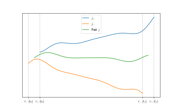
Sum all over pairs, $$ \sum_{\text{Pairs }j} $$ The pair $j$ is divided on $j_+$ and $j_-$ such that the midpoint of $\mathbf{r}_{j_+}$ and $\mathbf{r}_{j_-}$ is $\mathbf{r}=(q,p)$
Pair of Trajectories
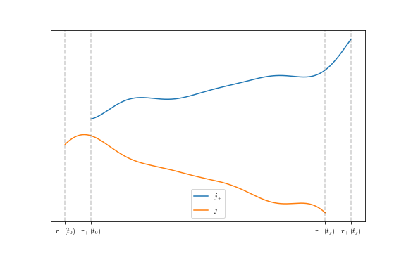
Midpoint
- Phase term, is divided on the action and maslov index
$$
\cos(S_j/\hbar-f_j\pi/2)
$$
- Action, $$ S_j=\frac{1}{2} \left(q_1(0)+q_2(0)\right)\left(p_1(0)+p_2(0)\right)-\frac{1}{2}(q_1+q_2)(p_1+p_2)+(S_1-S_2) $$
- Index of Inertia: Asociated with the matrix $\mathbb{M}_{j+}-\mathbb{M}_{j-}$ $$ f_j=\lambda_{pos}-\lambda_{neg} $$
- Stability Matrix If the trajectories are similar, they count more than different ones.
Symplectic Area

Caustics

Hyperbolic and Elliptic Pairs
The idea of taking
$$ \sqrt{|\det(\mathbb{M}_{j+}-\mathbb{M}_{j-})|} $$Makes indistinguishable the cases of the difference $>0$ and $<0$
Questions
- It is really not important the selection of the $+$ and the $-$?.
- Shall we have comparable sampling on both trajectories?.
- How can we manage small times if we have only one family?.
- When does it start being important?.
More on the Families.

Folding

Geometric Differences

How
We are appliying those concepts numerically and that is our main objective right now, so.
I am going to discuss in detail step by step, so that everything will become clearer.
Initial Distribution
We are not propagating a point (a $\delta$ function :The propagator). We are propagating a distribution.
In particular, we have been using coherent states (Gaussians.)
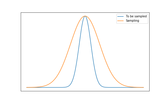
Initial Sampling
Even when we are propagating a particular distribution, we can use a different one just if it worths it.
We have been using the same gaussian to sample.
I think that if we are goung to use a gaussian, it should be one with bigger variance ($\sigma^2$)
Propagation
We propagate, independenly $N$ classical points in order to get, at the end, $\frac{N(N-1)}{2}$ points to construct the final distribution.
Classical Dynamics
We are using a symplectic 6th order method. Yoshida's Method!!.
Action Dynamics
We calculate the area enclosed by each classical trajectory.
Matrices Dynamics
The Matrices evolve with the Hessian matrix
$$ \Delta\mathbb{M}=\Delta t \mathbb{j}^T \frac{\partial^2 H(\mathbf{r})}{\partial \mathbf{r}^2} $$Reconstruction of the State
At the end, we may have two set of pairs, the Hyperbolic and Elliptic.
To reconstruct the state, we may have two different averaging strategies.
Averaging: Sampling
We do the following for each of both families.
As we do not sample the final points, there will be some of them that will have more final midpoints.
The final state (Wigner Function), must have a finite resolution due to it is numerically,
- Choose a resolution and region of interest. That defines a grid.
- We build two grids.
- For the propagation
- For the number of points on each cell.
- We normalize each final cell.
Averaging: Families.
We take the contributions of each family as equal.
Results
We strongly followed the procedure described before,